Note: This post is one in a series in which we examine the NCAA Tournament in some specific detail. Terms such as “the NCAA’s,” “Tournament,” “Tourney,” “March Madness,” or “March” refer primarily to the NCAA Tournament. Today’s installment looks at the relative importance of guards in the success of NCAA Tournament teams. Initial date of publication: 2/23/2024.
The purpose of this post is to examine if guards really do win in March. There are many claims college basketball fans make that are to the effect that good guards are primarily what matters in the Tournament. Some say that Cinderella runs are fueled mostly by great guard-play, others will extend this to better-seeded teams and say that Final 4 or National Championship teams tend to have elite guards. Others will take this idea even further and claim that interior-based teams which rely on post-play are destined for early exits due to their playing style, regardless of how good they were in the regular season.
Logically this doesn’t really make sense. If a team wins during the season with elite big-men who dominate in the post, why can’t it do so in the NCAA Tournament? After all, it’s the same 40-minute game in the Tournament as it was all year. Sure, maybe there are factors which make March basketball distinct (perhaps the games are officiated slightly differently, etc.), but for the most part the game is mostly the same game it was all season. We should see all types of playing styles work in March.
At the same time, the idea that guard-play is of heightened importance in March does seem to have a hint of truth to it. Looking back to last season’s Tourney (2023 NCAA’s), the Purdue Boilermakers Zach Edeys were a dominant regular season team which earned a 1-seed only to fall in the First Round to 16-seed Fairleigh Dickinson as 23-point favorites. FDU was a guard-oriented team1 that attacked Purdue from the perimeter. Although less-remembered, the 2023 Arizona Wildcats earned a 2-seed on the backs of a strong front-line (with weaker guards) and got bounced by a veteran Princeton team. Other forward-dominant teams also underachieved, whereas strong guard-play propelled Miami and Florida Atlantic to Final 4 appearances. 5’8 point guard Markquis Nowell single-handedly lifted K-State to an Elite 8, averaging 23.5 PPG and 13.5 APG on efficient shooting during his four-game run.
These anecdotes aside, it would be better if we could test to see if a guard-based style is better than a forward or interior-based style in March. But how could we do this? Let’s first by defining the problem and then introduce some terms that will help.
Guards to Posts – A Continuum
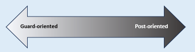
We will conceive of how teams play as a playing Style. Teams which feature guards for higher-than-normal minutes or rely on guards for higher-than-normal production will be classified as having a more guards-based style. Teams that rely on interior players to eat minutes or produce value will have a more interior-based style. This metric will be on a continuum. Certain teams will be very guard-heavy; others will be very interior-heavy. And in the middle there will be a bunch of teams with a more-balanced attack.
Terms
In discussing Style, we are attempting to understand where a particular team falls on this guard to post continuum. Style can be used to describe teams in other ways; such as fast vs. slow tempo, man-defense vs. defense with zone-concepts, and so on, but for our purposes in this post when style is used it is referring to how guard-dominant or forward-dominant a team is.
Relatedly, the two poles of this spectrum are guard-oriented and post-oriented. We will use other terms to describe these extremes, such as guard-based or guard-led or guard-dominant. The same terms will be used for the other pole, just with post or interior or forward used instead of guard.
Other terms will be defined when we get to them, but for the rest of the blog-post, keep the above continuum in mind when considering a team’s playing style.
Problem
Teams clearly play different styles, but how do we quantify these differences? What makes a team guard-based or forward-led? In order to classify teams into playing styles, we will need to get each team’s roster of players and classify each player into a certain position. From here, we will need to find a way to appropriately weight each player’s contribution to the team’s style. For instance, a team which has a slew of walk-ons that are all guards but relies on and plays a forward-heavy rotation is better defined as forward-dominant.
Data
We used Bart Torvik to collect the data, including player positional data. Torvik has already classified each player into a position based on his own algorithmic criteria. We will use his data and trust his insight on a basis from which to build our own analysis. Getting to player position, Torvik has classified players into 8 different positions. Using the 1-5, PG-C basketball-position concept, we will assign each position into a numeric role so that a quantifiable analysis can be achieved. These roles, and corresponding numbers are below.
Pure PG (1.0)
Scoring PG (1.0)
Combo G (1.6)
Wing G (2.0)
Wing F (3.0)
Stretch 4 (3.7)
PF/C (4.3)
C (5.0)
Some of these positions are hybrid-roles, so their numeric value is in between two positions. Torvik doesn’t list anyone as a pure PF (4), but many of these types are filled in the PF/C role with some getting a Stretch 4 role. Stretch 4’s aren’t traditional 4-men, but instead a hybrid between a 4 (bigger, good defensive rebounder) and Wing F (can hit outside shots).
We limited data to include only the 68 NCAA Tournament teams. We then gathered the following information from Torvik for each player that earned 10% of minutes for his team.
Player Name
Team
Role (position)
Min%
Box Plus-Minus (BPM)
Analysis
There are two different ways that team style can be calculated. One is what we call Style-Value. Style-Value (S-V) is when a team’s style is determined by how much value its guards bring in relative to how much value its interior players bring in. Value itself is calculated through using BPM and converting it to Wins Above Replacement (WAR)2.
The other way to determine team style is by Style-Minutes. Style-Minutes (S-M) calculates style by seeing how many minutes each position plays. Guard-heavy teams will often have multiple point-guards or play 4-guard lineups. Forward-heavy teams will be more traditional in terms of minutes allotment, often having two PF/C types on the floor and/or multiple Wing F’s at times.
These two styles have some correlation to each other, but it isn’t super-strong. We will consider both S-V and S-M in our analysis.
After normalizing style, we see that these teams were the most guard-like in terms of S-V among 2023 NCAA Tournament teams:
Penn State (-2.22 z-score, 10-seed, R32)
Baylor (-1.92 z-score, 3-seed R32)
Kansas State (-1.83 z-score, 3-seed, E8)
UCLA (-1.58 z-score, 2-seed, S16)
Miami FL (-1.28 z-score, 5-seed, F4)
Compare this list to the most guard-like teams in terms of S-M:
Nevada (-2.38 z-score, 10-seed, R64)
Fairleigh Dickinson (-2.20 z-score, 16-seed, R32)
Vermont (-1.70 z-score, 15-seed, R64)
Missouri (-1.69 z-score, 7-seed, R32)
Colgate (-1.53 z-score, 15-seed, R64)
The top list shows the teams that had elite guard-play, particularly relative to their forwards. The second list shows mid and low-major teams that relied on guard-play, although it wasn’t necessarily that they had elite guards. When we deal with teams in the NCAA Tournament, you have to understand that each team has different goals. For a top seed, making the Final 4 is a reasonable goal. For double-digits seeds, the more likely goal is just an upset win. So we will use both lists, S-V and S-M.
There were different ways to analyze the relative success of guard-oriented teams. We first looked to see how strong the correlation was between style and overall success. We looked for correlation between style and relative success (to seed). There was only a tiny correlation between guard-oriented style and team success, with S-M seeing stronger correlation than S-V.
After viewing correlation, we looked to see if the most guard-oriented teams fared better than the most forward-oriented teams. We filtered out only the styles that were a SD more guard-like than the mean or a SD more forward-like than the mean. Using S-V, we saw that the most guard-like teams won +2.1 games more than expected overall and the most forward-like teams won -3.6 games than expected overall. This was an advantage of 5.7 wins in favor of the guard-heavy teams and worked out to 0.3 wins per team. This isn’t a small difference.
We did the same thing for S-M, and got a difference of +4.4 wins for the heavy-guard teams relative to the forward-heavy teams (which worked out to about 0.2 wins per team). Again these results are in the direction of supporting the conventional wisdom regarding guards and March.
Next we looked at head-to-head results. Previously it was just records overall. But we wanted to see if having a heavier guard-based style was advantageous in head-to-head contests. In the NCAA Tournament there were 67 games played, and the more guard-based S-V team won 36 of these games. For S-M, the more guard-based team won 29/67. These results may seem conflicting, but they actually will lead us to a later insight.
Looking at head-to-head contests but considering Wins Against Expectation (WAE), we see that guard-oriented teams overachieve on the whole. Teams that are more guard-oriented than their opponents won +2.07 more expected games (S-V) or +2.43 more expected games (S-M).
If we look at head-to-head contests from the perspective of the underdog, we see that guard-based underdogs have a +1.80 WAE and forward-based underdogs have a -0.86 WAE in terms of S-V. This comes to a difference of +2.66 in favor of guards-based teams. Looking at the same thing from S-M, this is +1.57 and -1.76 WAE, or a difference of +3.33 in favor of guards-based teams. This doesn’t seem insignificant. Playing a guard-oriented style seemingly helps underdog teams overachieve in March.
We will look at final margin. Using S-V, we see that the more guard-based team is better than its opponent by 0.7 points per game. Using S-M, this is nearly 2.0 points per game better for the guard-based team. It makes sense that if the guard-based team is winning more than expected it is also doing better on expected margin.
So far in head-to-head results, we’ve been considering which team was relatively more guard-oriented to its opponent. But it isn’t like teams can schedule which style on the bracket they get to play against. They can, of course, determine the make-up of their own style. So what happens if we look at the relative success for guard-based teams regardless of opponent?
There were 30 games which faced a guard-oriented team against a forward-oriented team (using S-V). Paradoxically from what we’ve seen from earlier results, the results viewed this way favor forward-based teams. When we look at how guards-based teams fare against forward-based teams, the guards-based teams underachieve, with -2.53 WAE and -1.6 points per game (forwards-based teams are the inverse).
But when we do the same exercise on Style-Minutes, we see that guards-based teams overachieve by +6.05 WAE and are +5.1 points per game better than expected. This shows the importance of defining style. If we say a team is guards-based by looking at the relative value that team’s guards provide, it can give a whole different answer than if we say a team is guards-based by looking at its minutes distribution by position.
Making Some Conclusions
So where does this leave us? Is style important? Do guards win in March? And if so, how can this be used by coaches to gain competitive advantage?
Based on evidence so far, we would conclude not that interior-based styles are doomed to fail, but that guards-based styles are more likely to overachieve in March Madness. While there are weak correlations seen when we regress a team’s style against its success in the 2023 NCAA Tournament, when we filter out the most guard-heavy and forward-heavy teams, there is a clear bias in favor of the guard-heavy teams (relative to pre-Tournament expectation).
Likewise, when we view head-to-head results, the team that is more guard-oriented outperforms the team that is more forward-oriented on the whole. If we look at guard-based teams in head-to-head results (regardless of opponent-style), there is a contradictory answer based on if we base style upon value (Style-Value) or minutes (Style-Minutes). In all assessments, the Style-Minutes view showed stronger benefit for guard-based teams.
Overachievement is the key word. Guards-based styles displayed a better chance of winning when looking at pre-game or pre-Tournament expectation.
However, it isn’t clear how much coaches can use this to their advantage. Particularly because they do so already. Low and mid-major teams looking to pull the upset off are already more likely to be more guard-oriented than their favored opponent. In fact, of all the correlations we ran, the strongest one we found was between a team’s pre-Tournament computer strength and its style as a forward-based team. The best teams heading into the 2023 NCAA Tournament were more likely to be interior-based when compared to the average Tourney team.
But if low to mid-major teams gain a March advantage by playing guard-based styles, can this be neutralized by favorites looking to stave off an upset by playing small themselves? This is tough to say. In one sense, coaches of top teams are best to stick with the style that got them to a good seed in the NCAA’s, as they are still the favorite against the guard-based underdog. A favorite changing its playing style to become more guard-focused might help in some areas but hurt in far more areas (such as dominating the glass and paint). This trade-off might not be worth it.
Additionally, and this hasn’t been analyzed, but favorites might already be changing up their styles during March Madness, and this is partially to blame. Perhaps forward-based teams are going away from what got them to the Big Dance once things get tight in a early-round game, and this is being reflected in the data! We just don’t know.
We’ll close this section with examining the biggest upset in the 2023 Tourney. Purdue’s loss was blamed on its guards, and it strengthened the claim of those who say guards win in March. At the same time, this ignores how well Zach Edey played. Edey had 21 points, 15 rebounds, and 3 blocks. He drew fouls and made FDU work on the defensive end. While it wasn’t enough, had Purdue escaped the upset it would have been due to the team’s interior play. The point is that Purdue wouldn’t have benefited from changing up the style of play that earned it a 1-seed. Rather, it just needed its guards to not choke. The guards/wings went 5-26 from 3. Purdue had 16 turnovers but forced only 9. It lost the game on the perimeter for sure. But if Edey didn’t play, it wouldn’t have had the big advantage inside either, which would have made things worse.
More to Come
With the 2024 tournament coming up, it will be interesting to see if these patterns hold and if this information can be used in filling out a bracket. Picking guard-based top seeds to make deeper runs (using S-V) or double-digit upsets (using S-M) might be a successful strategy. We’ll fill out a few brackets using these principles and see how they do.
Beyond this, we will want to see if this is consistent across tournaments. 2023 had quite a few upsets, so this could have been the reason guards-based teams overachieved. Maybe 2019 (all but one S16 team was a 5-seed or better) or 2008 (all Final 4 teams were 1-seeds) will show the reverse. Maybe upsets or deep-runs are more memorable when a team is led by its guards, and this clouds our view on how style plays into Tournament success.
FDU was certainly guard-oriented from a minutes-played perspective, but in terms of player-value, FDU was not a team which featured even average guard-play during the 2023 season. FDU wasn’t good at all during the 2023 season, and entered the NCAA Tournament somewhere in the mid-200’s in computer rankings. If anything, it could be seen as having better forwards than guards as its interior players were less-bad than its guards. ↩︎
WAR multiplies BPM by Min% by a set # of games by a multiple to estimate a player’s contribution to team wins. ↩︎
After Jalen Wilson departed for the NBA and KU picked up 7’1 center Hunter Dickinson in the portal, K.J. Adams shifted his position from the 5-spot to the 4-spot in KU’s starting line-up. This shift has been seen on both ends of the floor. Offensively, he’s posting up less and making more plays on the perimeter as a creator (where he’s third on the team in assists). And while he doesn’t have what one would call “range,” he’s been making some mid-range jumpers and push-shots with Hunter underneath to rebound, which is what a traditional 4-man does when he is playing with a true 5-man.
But it is K.J. Adams’ defense which has been the most-valuable part of his game with his switch to the 4-spot. Last season, as someone primarily guarding the opposing 5-man at a height and length disadvantage, Adams was basically a neutral-value defender, finishing with a Per100 points-against bubble of -0.22. He gave up 12.7 points per 60 possessions (worst among the starters) as he had to battle inside. (Adams was able to benefit by having a slower player on him on the offensive end, so he did finish as a positive-value player overall (+0.49 per game)). In 2024, Adams is KU’s strongest defender, with a +5.01 Per100 value. And while his rebounding hasn’t really improved, he is giving up only 7.7 points per 60 possessions now that he’s guarding mostly wings and forwards. This defensive stinginess not only leads the team, but is close to the range of what KU’s best defenders have allowed over the past decades.
Since 2018, we have tracked defensive value at detailed-enough level to estimate which players were the best at not allowing points to be scored. This is seven seasons of data, including 2024. In this time, only three times has a player been a stingier defender than K.J. Adams this season. Marcus Garrett (2020 and 2021) accounts for two of these seasons. The other, which you wouldn’t probably guess correctly if you had 20 chances, was Isaiah Moss. While Moss didn’t rebound or force turnovers, he stayed close to his man and didn’t overhelp. Overhelping, particularly off wing shooters, is where many teams lose defensive value. Completely leaving one’s man should only be done to prevent an uncontested layup or wide-open 3 by a good shooter. Moss wasn’t overly athletic, but he had a high BBIQ as a veteran defender.
But back to K.J. K.J.’s value on the defensive end is estimated to be +5.01 points above that of a bubble-level player Per100 possessions. If we look at this from a per game ratio, then Adams is producing an estimated +2.91 points of defensive value above a KU-caliber replacement. According to current information, this would put him as having the 7th-best defensive season in the last 32 seasons (there have been 453 player-seasons in that time. K.J.’s 7th of 453).
That’s rather incredible. Whenever K.J.’s defense is talked about by fans, it’s often derided due to him not getting enough rebounds or having “short arms.” It’s true he doesn’t add value through rebounds or forcing turnovers. But he does an excellent job of not giving up easy scoring opportunities. He uses his strength to guard bigger players and his quickness to stay in front of guards. This versatility means he can easily switch positions 1-4 (and as we saw last season, can also play some against 5’s without being dominated). In turn, this forces teams to over-pass or take a less-than-ideal shot on certain possessions. All of this shows up in the numbers when we chart each defensive possession.
Note that these value estimates aren’t an exact science. Other sources don’t see him as having this much defensive value. Hoop-explorer doesn’t see much difference (although it relies on On/Off data which is very noisy and probably not wholly accurate). Evan Miya, which uses On/Off data and attempts to normalize the relative strengths of the other 9 players on the floor, has him as KU’s fourth-best defender. Without being overly critical, this seems to discount the on/off method for assessing player value. It isn’t K.J.’s fault if another teammate blows a defensive assignment when he’s in the game. While, with enough of a sample size, this “noise” would eventually even itself out (theoretically leaving you with just the player’s impact), it doesn’t seem to be the case unless there is a much larger sampling of minutes played. While K.J. has played 840 minutes so far, this only leaves 165 which he is on the bench. On/Off here isn’t really helping.
In 25 games this season, K.J. has posted positive defensive-scores in 21 of them. Teams aren’t attacking him much (like they would last season if they had a capable big). This means he’s doing his part. KU’s had defensive lapses, particularly among ball-screen coverage, but this is mostly due to Hunter being out of position (KU would do better to drop him rather than have him hard-hedge) or a separate wing/guard not being good at rotating over. K.J.’s fewest minutes in a game came against Chaminade, after he arrived following the death of his mom and didn’t start. He wasn’t expected to play, but did get on the court for 26 minutes and produced a small positive amount of defensive value. Self clearly wanted him on the court despite the opponent being a Division II team. This is further evidence that his defense warrants playing time, and is thus valuable.
All KU fans agree that Hunter Dickinson is a skilled and valuable offensive player. Some argue that Dickinson’s defensive deficiencies (they take for granted he’s a poor defender) severely undercut his offensive value. This post will examine Hunter’s defense by comparing him to other players on this season’s roster as well as KU centers in seasons past.
A player can be a plus defender in one of two broad ways. He can either do so by limiting the amount of points his man scores or he can be a good defender by getting the ball back for his team (such as rebounding). Note that these are related. A defender getting a rebound is also preventing his man from scoring on a putback attempt. The very best defenders are good at both aspects–they limit their opponents’ good looks and they get the ball back for their team.
Applying this to Hunter in particular, we want to examine how often he is most responsible for the other team scoring (compared to others) and how often he wins possession back through a block, rebound, steal, or forced turnover (compared to others).
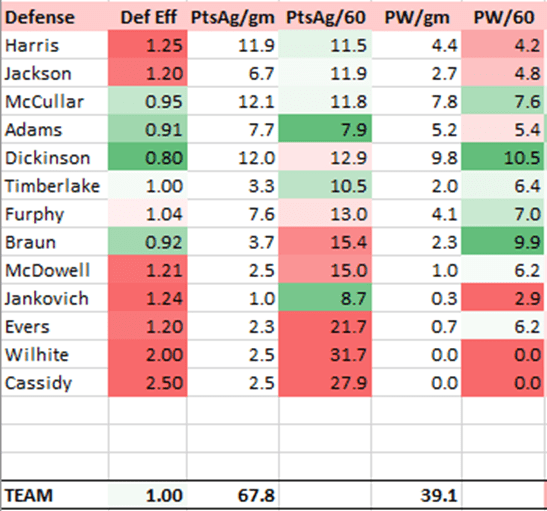
Using the Charting methods, we calculate that Hunter has allowed 276 points in 23 games this season (12.0 ppg). When we convert this to a 60-possession basis, this comes to 12.9 per 60. This conversion is done to compare Hunter to other players.
Next, we can count the number of stops KU gets because Hunter gets the ball back through either a block, rebound, steal, or forced turnover. As rebounds are most common way a defense gets the ball back after a stop, Hunter’s importance is mostly by being a great rebounder. He averages 10.5 possessions “won” over 60 defensive possessions.
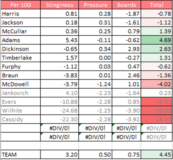
For the 2024 team, we can consider this table.
Looking at the Points Against Per 60 column, this shows that Hunter (allowing 12.9 per 60) is worse than the other starters save Furphy (13.0 per 60). However, he is better than his backup Parker Braun (15.4). Additionally, only K.J. Adams (7.9) is significantly better than Hunter at disallowing points. Harris and McCullar have been in the middle-of-the-pack.
If we move to the far-right column, we see possession winners per 60. In this case, Hunter is clear-and-away the best at getting the ball back following a miss or through a forced turnover.
When some think of defense, they mostly consider the first aspect of this, or on-ball defense. And this aspect is very important. Not getting beat, not fouling, closing out on shooters, forcing a player to pick up his dribble and pass, etc. are all ways a defender can make it more difficult for the opponent to score. But the second aspect, or coming away with the ball, is also important. First-shot defense that doesn’t win the ball back will lead to second and third chances that can allow points. A player who might not be a great first-shot defender can still add value if he prevents opponents from getting second-chances. So, we need a way to combine these elements of defense into one number that estimates player value.
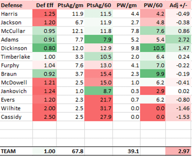
Using theory regarding the relationship to points and possession in basketball, we can calculate how valuable these defensive metrics are. We will now include the defensive value metric in the final column of the table.
This final column estimates, in points per game, how valuable a certain defender is when compared to a replacement (bubble-level) player. Due to his stingy on ball-defense, K.J. has graded out as KU’s best overall defender. But the second-best defender has been Hunter Dickinson–not because he is always great at disallowing points–but because he limits teams’ second-chances. Imagine KU without Hunter on the floor. Teams would get many more baskets through second-chance opportunities.
This is common among bigs in today’s game. The prevailing offensive strategy involves getting opposing 5-men away from the basket (to clear driving lanes and cutting angles). As Hunter is involved in ball-screen defense and plays on the perimeter at times while on defense, he is often put in situations where he can find himself out of position. This leads to breakdowns, rotations, and open shots for opponents. But this isn’t always what happens. Other times he defends fine, and the possession ends with a missed shot that he has a great chance of rebounding due to his height and good rebounding technique.
We can break down the defensive value provided by 2024’s roster further, using 3 categories and a Per 100 possession basis. These three categories are: Stinginess (or points allowed), Pressure (forced turnovers/steals), and Boards (rebounds).
Hunter’s Stinginess score is below-bubble, but at -0.65 points we estimate that it only costs KU less than a point per 100 possessions. His Pressure (+0.34) and Boards (+2.93) make up for it, leading him to be a +2.63 player over 100 possessions. This is nearly 4 points better than his backup, Parker Braun has been. He is also better defensively than all other players save K.J. Far from being a liability, Hunt’s been a valuable asset for the 2024 defense.
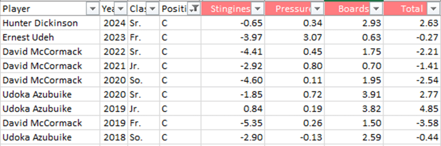
We can also compare Hunter to 5-men of past seasons. Below is a table of all players labeled center who’ve played 10% of minutes on the season or more since 2018. This includes 9 player-seasons.
Here we see a pattern. 8 of the 9 centers on this list have negative Stinginess value, showing that they are allowing points more often than the average defender. This makes sense. Teams are attacking the slowness of the big men to find an advantage that leads to points. However, once we move right, we see that the 5-men can Pressure and Board better than average. So while your guards are likely to be better at preventing open shots, they struggle to get the ball back. Hunter’s rebounding better than any recent center not named Udoka. Additionally, his overall defense is 3rd best out of 9 centers since 2018, again only behind 2019 and 2020 Azubuike.
We can expand this more, just with less detail. Since 1993, there have been 192 players who have played at least 40% of the team’s minutes during the season. Of this 192, only 45 have had a per game defensive value as good as Hunter’s having this year. He’s objectively around the 76th percentile of defensive players in recent Kansas history. Ignore people who don’t know how to track defensive value and fail to consider all relevant factors of defense.
In addition to tracking individual defense, we can confirm these general findings by looking at proxy metrics. One such metric would be points in the paint. This season, for reference, KU’s offense is averaging 40.1 points per game from paint scoring. That’s what a good offense does. A large chunk of this is from Hunter (although K.J. and Kevin are also doing well at the rim). So let’s use KU’s offense as a comparison to KU’s defense. The thought would be that if Hunter’s offensive-value is being wiped away by poor defense, then KU will be allowing nearly as many points in the paint as it is scoring.
This isn’t the case at all. KU is only averaging 25.8 points per game in the paint. This is a difference of 14.3 points, which is more than the overall point difference (10.9). KU is winning points in the paint but losing in all other areas (that is FT’s + 3’s + 2’s outside the lane). This is just further confirmation of Hunter’s value.
KU’s 24-point win against a hapless Oklahoma State team last night boosted its KenPom rating to +22.27, which is good enough to be 14th overall as of January, 16. There’s been some debate about the accuracy of KenPom’s system, as it appears to reward teams more for blowing out bad teams than beating good ones in close games.
Without getting into a longwinded opinion about what KenPom is “about,” I wanted to explore what I call a team’s “Game Score” and see if, in theory, a good team could improve its KenPom rating by scheduling easier.
First, let’s discuss Game Score. Game Score is the attempt to quantify how good a team’s game is by adjusting the final margin depending on the opponent and location. That is, a 10-point home win against a team ranked 250th would be much less impressive than a 10-point road win against a team ranked 25th. Game Scores tie to KenPom’s ratings in a few ways. One, they use KenPom’s Adjusted Efficiency numbers to determine opponent strength. Two, they are linear or rely on a linear system to compare game performances, just like KenPom. If a team is projected to win by 10 and it wins by 15, the team’s KenPom rating will climb. However, the hypothesis is that a good team can have a higher average Game Score (and in turn elevated KenPom rating) by playing an easier schedule, because it is easier to “juice” a winning margin in games already in hand. When playing an overmatched opponent, leaving in the starters just a few extra minutes can be the difference between say, a 25-point win or a 30-point win. The Game Score will increase by 5 points as well, as the opponent adjustment is already baked-in.
To test this, we will use KU games over the past few seasons. Kansas has been consistently good over this period and is a good team to use. My theory is that there will be an inverse relationship between Game Score and opponent quality. Remember, in theory, opponent quality should neutralize the effect of the actual margin, making Game Score independent of opponent quality. Does reality show this to be the case?
KU has played 229 official games since the beginning of the 2018 season (November 2017). These games have been played against a variety of opponents, some good, some not. Will it be easier to produce higher Game Scores against worse opponents than better ones?
Results
There was a small inverse correlation between opponent quality (opponent’s KenPom rating) and Game Score. While this might seem insignificant at first, it can make a difference when we look at the results.
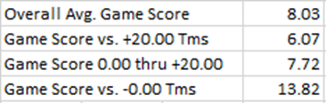
Since 2018, KU is averaging a +8.03 Game Score. This just means that KU is beating its opponents by an average of about 8 points more than a typical bubble-team would. When we break it down into buckets by quality of opponent, we see a clear trend. Against the best teams in the country, those with a +20.00 KenPom rating or higher (roughly your top 15 to 20 teams, depending on year), Kansas is only producing a Game Score of +6.07. Against decent to okay teams, those with a KenPom rating from 0.00 to +20.00 (corresponding to ~ 20 – 180), Kansas is producing a Game Score of +7.72. The best Game Scores are those against inferior opponents, those with a negative KenPom rating or who are worse than the average D1 team. KU is, on average, +13.82 in these games.
What this shows is that, over the past 7 seasons, KU is more likely to climb in KenPom when it plays games against easier opponents. As KenPom is trying to account for opponent strength already, it does give strong credence to the idea that teams who play a weaker schedule are juicing their KenPom scores by doing so. This would apply to teams like Gonzaga in past seasons, but also to the non-conference schedules of Houston and BYU in 2024.
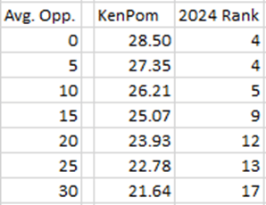
What we’ll next show is the expected KenPom ratings/rankings for a hypothetical Kansas team that is as strong as the average KU team since 2018.
The first column looks at the average opponent KenPom rating, and then projects this hypothetical KU team’s KenPom rating. The next column is the KenPom ranking for additional context. We see that as the average opponent score climbs, the KenPom rating/ranking for hypothetical Kansas worsens. A schedule of 0.00 opponents would allow Kansas to juice its score all the way to a #4 ranking this season. If it played a schedule against top-tier opponents, like it will in stretches of conference play, this ranking drops out of the top 10.
An additional level of data relates to the 374 games played since the 2014 season. KenPom provides pregame point differential estimates as well as winning percentage estimates (effectively odds). With this info, we can make the prediction that KU will “overperform” in easier games compared to games where the margin is expected to be smaller. In the 90 games where KU had a 90% chance or greater of winning, that is the easier games, KU has outperformed its expected KenPom margin by +2.41 points per game. In the 284 other games, the games expected to be closer, KU is outperforming KenPom expectation by only +0.49 points. This accounts for a difference of 1.92 points per game, or roughly 2.74 AdjEm on KP. Again, this is further confirmation that good teams can juice their KenPom ranking by playing an easier schedule.
Relevance to the 2024 season
This is relevant to Houston, a team which has a non-conference average opponent rating of -1.21 (215th), as well as BYU, a team which has a non-conference average opponent rating of -5.01 (307th). For Houston, if we look at its 6 games against Top-100 opponents, we note that it has performed where a team with a KenPom score of +27.39 would, or nearly 5 points lower than its current (juiced) +32.31 rating. Only looking at conference-play against Top-100 opponents, a small sample size for sure, its comparable KenPom score is +21.82.
BYU’s 7-game slate against Top-100 opponents has it 4-3, with an estimated KenPom rating of +20.14. This is the difference between 9th or 20th. Again, we’re seeing evidence that a team’s KenPom rating is aided by blowing out inferior opponents. For both Houston and BYU, their overall schedule strengths will get better, meaning that what KenPom says about them in March will include more data against strong opponents. As both are good teams, one shouldn’t write either of them off. But what Purdue (best overall schedule) or Wisconsin (surprise team around BYU’s ranking yet has a solid SOS) have done so far should give them the nod ahead of teams similar to them in the KenPom totem.
We can use Bart Torvik’s filter tool to explore this phenomenon more. While Torvik has different inputs than Pomeroy, he is attempting to do the same thing. If we only look at opponents that are Quad 2 or better (using NET), we see that Purdue is best (and better than Houston by almost 7 points per 100 possessions. Houston is slightly better than Purdue accounting for all games). Similarly, BYU is 26th best when playing top opponents, as opposed to 7th when all games are included.
Determining the Best Teams
So, who is the best team in the country? How much should advanced metrics be considered? Keen observers will note that, in criticizing KenPom’s rating for Houston or BYU, I still used KenPom numbers. That highlights the inherit difficult of any ranking system. Rankings are relative, they depend on how good others are. KenPom’s value is that the system provides a fairly accurate look at each team’s relative strength compared to any other of D1’s 362 teams. If a system makes adjustments to remove Houston or BYU’s blowout wins, it underestimates their strength relative to a team outside its Top-150. So for any advanced rating system to be most accurate, not just accurate among a certain range of teams, it needs to include all game data.
For the purposes of college basketball, the only important rankings are those of the selection committee preparing to set the field for March Madness. The selection committee gets criticized, sometimes rightly, but those who want to do away with the committee and institute a computer-based ranking system (such as WAB) are completely misguided1. Even the most well-known advanced rating system has noticeable flaws. The committee’s focus on strength of schedule (dissuading teams from scheduling cupcakes in the non-conference to artificially boost their overall record) appears to be a good thing. It looking at a team’s best wins or worst losses will also filter out noise, allowing a better comparison between teams near each other on the seedline.
Summary
Teams have an easier time improving their advanced metrics by playing a softer schedule that allows for blowout wins. Teams that’ve achieved high rankings by playing a strong schedule should be seen with less skepticism than teams that have mostly blown-out lesser opponents. Still, let’s not be overly critical toward systems like KenPom, which are trying to rank all teams (not just the top 50 or whatever).
The only real ranking that matters is the NCAA Committee’s “S-curve” on Selection Sunday. While the committee does get things wrong, it has avoided errors by not adopting a metric-dependent system like some of its detractors demand.
1- Gasaway states the following in his appeal to do away with the Committee: “Whether your preferred metric is wins above bubble (WAB), strength of record (SOR), or something similar, any team’s record can be evaluated according to how difficult it would be for other teams to achieve the same result against the same opponents in the same venues. Wins are the key metric, as they should be, and teams can excel whether their schedules turn out to be grueling or unexpectedly soft.” (Links in original).
His assumption is faulty. We cannot confidently say that WAB or SOR are accurate enough when its been shown that the advanced metrics themselves understate how easy it is for a good team to blowout a bad one. This isn’t to say that WAB or SOR cannot be tools that an informed committee uses, but a committee-less NCAA Tournament selection process that only looks at a computer metric would reward teams that dominate against a light schedule and punish teams that take some lumps in tough conferences but still finish around 19-12.
Wins Above Replacement (WAR) and PAB (Points Against Bubble) have similar concepts and therefore the lists will be similar. Both are attempting to rank the careers of all KU players since 1993 to see which Jayhawks have been the most valuable for the program. The differences stem from the benchmark player upon which value is judged. In WAR, the “replacement player” is basically an average D1 player whereas in PAB, the “bubble player” is a player whose value makes a bubble team no more or less likely to make the tournament. In other words, a bubble player is a much higher standard than a replacement player.
So why the two lists? Which list is more valid?
At the top of the list there isn’t a ton of difference as guys like Raef LaFrentz easily clear the bubble level just as they clear the replacement level. It is further down the list where this distinction matters. Take Jeff Boschee for instance. Boschee was a four-year starter who is currently 57th in career WAR but 168th in PAB. Boschee was better than a replacement player but not better than a bubble-level player for the majority of his career1.
These are widely different rankings, leading to the follow-up question, which list is better? Well, it depends. Being a better-than-bubble player is crucial for KU to approach the success demanded of it. So we would normally lean with PAB. However, sometimes players who are not quite at bubble-level (but still solid enough to be above replacement level) are required to play heavy minutes due to roster issues or coaching decisions, and it wouldn’t be fully accurate to list these players below low-minutes-played players because of this. Boschee serves as a great example. He was certainly a below-KU-average guard given the minutes he played, particularly as an underclassman. But he was still valuable because he was better than the alternatives at his position.2 This is where WAR can be a better metric.
There is a third way to measure that is present, namely Per100 (possession) against bubble value. This is the third column on the second table. This shows the value the player provided while on the court, effectively ignoring playing time. Be aware of the limitations of this measurement. One, if we sorted by this list we’d include walk-ons at the top who graded out very well in very small, unimportant minutes. Two, durability is an important feature inherent to both WAR and PAB but ignored in Per100 value. A player who generates high value per possession but does not stay healthy throughout the year may not help the team as much as someone who can play a full schedule and heavy minutes at a lower value. A four-year player with solid value (like Marcus Garrett) will provide more value to KU than an elite one-and-done (like Joel Embiid).
Both WAR and PAB are useful lists but cannot be considered in isolation. If we are looking toward the top of the list, PAB is the better measurement. It estimates how many points a player gave to Kansas above that of a bubble-player over his career. Toward the middle and bottom of the list, WAR becomes the better mark. Clearly role players with sub-bubble (but above-replacement) value are preferable to the walk-ons. Lastly, Per100 can add some more context but we must be careful to not over-emphasize this measure as it is total value, not per possession value, that is most important when determining this ranking.
Boschee’s only above-bubble season was his senior year in 2002. ↩︎
Marlon London and Jelani Janisse are examples of other backcourt players on the roster in the Boschee-era. KU’s backcourt talent depth was quite thin during Boschee’s first three seasons at Kansas. ↩︎
Dajuan Harris’s last 15 games of 2023 vs. Dajuan Harris’s first 15 games of 2024:
Stat
2023 – Last 15 Gms
2024 – First 15 Gms
PPG
11.3
6.9
eFG%
62.8%
48.5%
TS%
61.5%
471.%
APG
5.8
7.1
A/TO
3.0
2.6
SPG
2.6
1.2
RPG
2.9
2.2
ORtg
109.6
102.4
Pts AB +/-
+48.39
-44.98
PPG +/-
+3.23
-3.00
Per 100 +/-
+5.14
-4.84
The numbers speak for themselves. Another notable thing is that KU’s average opponent had a KenPom rating of +17.10 over last 15 games in 2023 compared to +4.77 over KU’s first 15 games in 2024. Juan’s drop in production and efficiency has come against weaker foes.
The last three numbers are the value scores, first in total points against bubble, and then rated in per game and per 100 possession bases. These numbers account for opponent strength as well as deeper defensive metrics such as points allowed (Harris is allowing 12.4 points per game in 2024; it was 10.0 over the last 15 in 2023).
Aside from assists, Harris has gotten worse in every facet of the game. But even with assists, his increase in assists has come with a greater increase in turnovers, meaning his overall “ball-handling” value has worsened.
This and That
The following bits of info relate to the 2024 season through KU’s first 15 games.
Johnny Furphy’s defense has been better than his offense. Per 100 possessions, Furphy is about -1.03 points to a bubble player on offense and 0.00 to a bubble player on defense. Furphy is shooting well, but he relies on assists to score and turns it over far more than he creates offense for others. Defensively, his coverage score is not terrible and he rebounds at an acceptable clip.
Elmarko Jackson has posted 3 above-bubble offensive games, or 20% of the 15 he’s played so far in his KU career. And 2 of these came in KU’s first 2 games. What’s giving him any playing time at the moment is his defense. Jackson has produced 10 positive defensive outings this season (67% of games).
K.J. Adams is KU’s best defender right now, posting a +2.23 average defensive game score. This is far better than his 2023 season, which was negative (-0.10). Adams’ improvement on defense is in large part due to him defending less in the post as an undersized 5-man, his role last season. Offensively, Adams has seen a slight decline from ’23 to ’24 (+0.60 to +0.44).
Kevin McCullar’s value-score improvement from last season to this season, on a per game basis, is +3.98. This is better than Jalen Wilson’s improvement from ’22 to ’23 (+3.34), Ochai Agbaji’s improvement from ’21 to ’22 (+3.09), and Christian Braun’s improvement from ’21 to ’22 (+3.83). The largest season-to-season jump on record is Frank Mason’s ’16 to ’17 improvement (+4.52). Thomas Robinson from ’11 to ’12 was +3.67. Tyshawn Taylor from ’11 to ’12 was +3.65. Other large jumps in the past include Raef LaFrentz from ’95 to ’96 (+3.67), Keith Langford from ’02 to ’03 (+3.59), and Drew Gooden from ’01 to ’02 (+3.41). There have certainly been other great career developments of steadier growth, but in terms of having such a large leap in value production in consecutive years, what McCullar is doing this season is very special.
Hunter Dickinson’s two worst value-score games (-10.40 vs. Marquette, -6.23 at UCF) have coincided with both of KU’s losses. Through 15 games, Hunter is currently KU’s second-most valuable player this season, but is neck-and-neck with Kevin for this distinction. If both can finish the season above +5.00 per game, they’d be the first duo since the Morris twins in 2011 to do this for a Kansas team.
Jamari McDowell has not proven to be the answer to the team’s poor wing play. The freshman has produced the worst Per 100 value of any scholarship player, at -7.91. After some initial stingy defense, Jamari has gotten scored on quite frequently in limited minutes. At best, McDowell is only going to be a role player and defense-first guy this season.
Parker Braun has been KU’s 5th-best player, and might warrant more court time. He is athletic and experienced. His value scores through 15 games have been 7 positive, 7 negative, and 1 right at 0. While he is at Kansas primarily to back up Hunter, there have been a few moments where Self has gone “small” and played Adams as the 5 when Hunter is sitting. But this leads to more minutes for guys (Jackson, Harris, Timberlake) that aren’t playing as well as Braun has, and haven’t shown enough offensive firepower to compensate the loss of not having a true center inside. Parker isn’t necessarily someone who will win you the game, but he is someone who can keep you in it until Dickinson can return.
The 2023 portion of the 2024 regular season is wrapped up. KU went 12-1 during this non-conference stretch, a good result given the quality of opponents it faced. Using the NCAA’s Net Rankings, KU went 3-1 in Quad 1 games and 1-0 in Quad 2 games. Extrapolate that type of performance out over the rest of the season, and the Jayhawks will cruise into March as a 1-seed. But, this may not be that likely given a few concerning trends.
Best Game, Worse Game
Using a very similar concept to how Ken Pomeroy rates his teams, Charting the Hawks using a point margin difference to rate individual players or games. For CtH, a comparison level of a bubble-team is used to judge how well a player or the Kansas team itself is performing. This is in point differential (or margin) in comparison to a bubble-level mark. For instance, if we’d expect a bubble-level team to beat KU’s current opponent by 10 points (after accounting for location), and KU wins by 18, we’d say that KU had a “game score” of +8.00. This +8.00 score would also equal the net of all Kansas players’ individual game scores, as the system is breaking down each player’s value as a portion of the total team score.
This system is not perfect, but it does have the benefit of being easy(ish) to calculate and understand. In the non-conference, KU’s best game (relative to opponent) was its first one against North Carolina Central. KU’s game score was +24.04, meaning it won by 24 more points than a bubble-team would have expected to. On the flip side, KU’s 8-point win against Eastern Illinois garnished a game score of -15.43, indicating that the actual single-digit margin Kansas won by was about 15 points worse than what a bubble-team would have expected to achieve.
Looking at individuals, KU’s best performance in a game was Hunter Dickinson’s +17.63 margin against Tennessee. Dickinson scored 17 points in that game, but defended great (only allowing 3 points) and rebounded at an elite level, coming down with 20 official rebounds. The interior was owned by Kansas, forcing Tennessee to jack up 33 3-point shots, only to make 9. KU scored 20 more points than the Vols inside the arc that game.
Hunter also has KU’s worst individual performance. It occurred the night before the Tennessee game, against Marquette. Hunt’s score was -10.16 points, indicating a bubble-level player (think average player on a bubble-team) would be expected to play this many more points better against that opponent. In Dickinson’s case, it was the play of Oso Ighodaro which contributed to such a poor game score. Hunter had his worst defensive performance as Ighodaro scored 21 points that night, much of it against HD. In total, Dickinson would give up 26 points to Marquette while grabbing a season-low 8 rebounds.
While this was Dickinson’s worst game, on the season Hunter has been tremendous. Through 13 games, he is adding an estimated 5.35 points per game above bubble, second only to Kevin McCullar at +5.89. The team, as a whole, is averaging only +5.30 points per game above bubble. While the Hawks are 12-1, their point margins haven’t been as good as we’d expect.
Grading Projections
Before the season, KU was projected to have an average game score of +8.51 (vs. +5.30 in reality). This 3.21 point per game difference could be the difference of a win and loss in multiple conference games. In fact, KenPom’s predicted scores for KU’s conference games show 14 games out of 18 to finish within single-digits. KU having underachieving its desired margins so far is a sign of concern, as point margin has predicative implications. This doesn’t mean Kansas can’t improve. To see how, let’s break down KU’s performance to the player level.
This table shows each player’s 2024 projection and actual play through 13 games in points per game.
Player
Pre-Season Proj
Current Actual
Dajuan Harris
+2.50
-2.79
Elmarko Jackson
+0.10
-0.89
Kevin McCullar
+1.71
+5.89
K.J. Adams
+0.93
+2.33
Hunter Dickinson
+5.18
+5.35
Nicolas Timberlake
+0.32
-1.82
Johnny Furphy
-0.84
-0.12
Parker Braun
-0.39
-0.37
Jamari McDowell
-0.72
-1.07
TEAM
+5.30
+8.51
In PPG, individual scores won’t add up to TEAM due to walk-on scores missing
While there is still a lot of season left, there have been quite a few players with far different scores than their preseason predictions. Dajuan Harris has been the worst, performing over 5 points worse per game than his projection. Nicolas Timberlake and Elmarko Jackson have also been worse than expected, although Jackson has performed to his preseason expectation over his last 8 games (thanks to his defense). But KU’s guards are what’s holding the team back.
On the flip side, Kevin McCullar has overshot his preseason forecast by more than 4 points a game. McCullar is the Jayhawks’ leading scorer, having hit double-figures in every game this year. His low output was 12 against Kentucky, but this came in his first triple-double performance of the season (he’d add another against Chaminade). Fellow returnee K.J. Adams is defending at a conference first-team level after making the switch back to the defensive perimeter this season. His value score has easily exceeded his value score last year, as he’s also finding new ways to score. Newcomer Hunter Dickinson has hit his lofty preseason expectation of over 5 points of value per game. His backup, Parker Braun, is right at his incoming projection. The other wings, Johnny Furphy and Jamari McDowell, are within range of their projections, but Furphy has certainly played the better of the two.
If we look at where KU can get more value, it’s clear that the wings and interior players are tapped out. Not much more can be expected from Hunter or Kevin. KU needs its guards to start playing better on a consistent basis. This starts with Dajuan Harris. After reaching a season low -3.64 points per game against bubble mark after the Mizzou game, an unprecedented mark for a starter, Harris has responded with 2 positive games over his last 3. Against Wichita State, Harris had his best performance mostly due to a solid defensive game. It’s on this end where Harris has been especially disappointing. Dajuan was the conference defensive player of the year last season; in the 2024 season he’s worse than 1.08 points per game compared to a bubble-level defender. Had he been generating a bunch of offense to compensate, this would be more understandable. But his offense has been the worst it’s ever been, due to limited scoring and poor shooting rates on his floaters and runners.
With KU performing around 3.21 points worse per game than expected, and some of that due to the play of the walk-ons, we can essentially single out one single culprit as to why KU’s margins aren’t as strong as they were expected to be. This culprit is Dajuan Harris. While Timberlake and Jackson have been less valuable than expected, their poor play has been covered by the strong play of McCullar and Adams. Had Harris only played at a bubble-player level, or around 0.00, KU would be hitting its preseason expectations and be about fifth on KenPom (instead of 13th). Furthermore, Harris is KU’s point guard. He is the only one with the pace and ball-handling to run the team effectively at this point. KU can mix and match on the wings, using Furphy and McDowell when Jackson or Timberlake struggle. It doesn’t really have a Dajuan replacement and thus needs him to perform.
New Projections
The new projections use the actual play over the first 13 games along with the preseason projections in a weighted fashion. We should expect a player to trend back toward his preseason projection. These numbers are just a math equation; there’s been no new analysis involved at deriving them.
Player
Pre-season Proj
Current Projection
Dajuan Harris
+2.50
-0.63
Elmarko Jackson
+0.10
-0.49
Kevin McCullar
+1.71
+4.18
K.J. Adams
+0.93
+1.76
Hunter Dickinson
+5.18
+5.28
Nicolas Timberlake
+0.32
-0.95
Johnny Furphy
-0.84
-0.36
Parker Braun
-0.39
-0.38
Jamari McDowell
-0.72
-0.88
TEAM
+8.51
+6.61
In PPG, individual scores won’t add up to TEAM due to walk-on scores missing
Worst Case, Median Case, Best Case Scenario
These scenarios are updated from the preseason ones. Also included after each scenario is a look at what that team’s Final 4 chances would be, using historic F4 percentages by seed-line.
The new team scenarios are as follows. The actual worst case is of course an injury to Kevin or Hunter, but barring that improbability, a worst-case scenario that sees KU maintaining its full roster would be that KU’s guards never develop and teams continue to double on Hunter to make the others beat them. In this scenario, teams also focus their defensive energies on denying the ball to McCullar. While I can’t see KU failing to win all but a few of its home games, it could hit a tough spell during conference play on the road and rack up multiple losses in a row. For seeding purposes, KU could fall to a 5 or 6-seed if it can’t get necessary plays from its back-court. F4 chances: ~5%.
The most-likely scenario, or median case, would be that Jackson and Harris pick things up, building off of recent good performances, and start to produce for the Jayhawks during conference play. Harris doesn’t seem far off, and Jackson has been a legitimately solid defender whose offensive game has started to come around (had a career high 12 points vs. Wichita State). In this scenario, KU continues to win close games, loses a few close games, but also gets a bit better on the margin front which helps it out. KU earns a 2 or 3-seed and has a good chance to make the second weekend given its experience and talent. F4 chances: ~15% (Bart Torvik puts KU’s F4 chances at 10.4% as of 1/2/2024)
The best-case scenario is that KU gets the Dajuan Harris of last season to go along with the excellent play of its wings and front-court. Jackson fills his role nicely as a solid transition player and defender, Furphy and Timberlake come off the bench to knock in 3’s, and Braun and McDowell continue providing solid energy so the team can play 9 and stay fresh. In this scenario, KU establishes its dominance during conference play and fends off the new teams with strong efficiency marks in non-conference play. KU then goes on to earn a 1-seed in the NCAA’s and puts itself in a good position to make a Final Four run. F4 chances: ~35%
The following table projects the career majors for 100 top and notable golfers. This projection was made as of January 1, 2024. The ages listed reflect the golfer as of this date.
Player
Age
Current Majors
Projected Majors
Est’d Total Majors
Tom Kim
21
0
2.23
2.23
Scottie Scheffler
27
1
2.17
3.17
Collin Morikawa
26
2
1.77
3.77
Gordon Sargent
20
0
1.60
1.60
Viktor Hovland
26
0
1.55
1.55
Jon Rahm
29
2
1.54
3.54
Jordan Spieth
30
3
1.43
4.43
Sungjae Im
25
0
1.42
1.42
Rory McIlroy
34
4
1.08
5.08
Joaquin Niemann
25
0
0.90
0.90
Rasmus Hojgaard
22
0
0.80
0.80
Justin Thomas
30
2
0.72
2.72
Xander Schauffele
30
0
0.69
0.69
Patrick Cantlay
31
0
0.69
0.69
Cameron Smith
30
1
0.61
1.61
Cameron Young
26
0
0.60
0.60
Brooks Koepka
33
5
0.56
5.56
Matt Fitzpatrick
29
1
0.55
1.55
Sam Burns
27
0
0.54
0.54
Nicolai Hojgaard
22
0
0.49
0.49
Will Zalatoris
27
0
0.44
0.44
Hideki Matsuyama
31
1
0.43
1.43
Bryson DeChambeau
30
1
0.41
1.41
Ludvig Aberg
24
0
0.37
0.37
Ryo Hisatsune
21
0
0.31
0.31
Tommy Fleetwood
32
0
0.30
0.30
Min Woo Lee
25
0
0.29
0.29
Sahith Theegala
26
0
0.27
0.27
Tyrrell Hatton
32
0
0.27
0.27
Si Woo Kim
28
0
0.21
0.21
Jason Day
36
1
0.21
1.21
Patrick Reed
33
1
0.19
1.19
Mito Pereira
28
0
0.19
0.19
Corey Conners
31
0
0.18
0.18
Wyndham Clark
30
1
0.18
1.18
Tony Finau
34
0
0.16
0.16
Cameron Davis
28
0
0.16
0.16
Beau Hossler
28
0
0.15
0.15
Denny McCarthy
30
0
0.14
0.14
Rickie Fowler
35
0
0.14
0.14
Max Homa
33
0
0.13
0.13
Russell Henley
34
0
0.12
0.12
Aaron Rai
28
0
0.11
0.11
Christiaan Bezuidenhout
29
0
0.11
0.11
Justin Suh
27
0
0.11
0.11
Emiliano Grillo
31
0
0.11
0.11
Shane Lowry
36
1
0.10
1.10
Dustin Johnson
39
2
0.10
2.10
Talor Gooch
32
0
0.10
0.10
Patrick Rodgers
31
0
0.09
0.09
J.T. Poston
30
0
0.09
0.09
Brian Harman
36
1
0.09
1.09
Taylor Montgomery
28
0
0.08
0.08
Abraham Ancer
32
0
0.08
0.08
Lee Hodges
28
0
0.08
0.08
Adam Svensson
30
0
0.06
0.06
Sepp Straka
30
0
0.06
0.06
Harris English
34
0
0.06
0.06
Vincent Norrman
26
0
0.06
0.06
Adrian Meronk
30
0
0.06
0.06
Keegan Bradley
37
1
0.06
1.06
Harold Varner III
33
0
0.05
0.05
Jordan Smith
31
0
0.05
0.05
Byeong Hun An
32
0
0.04
0.04
Adam Schenk
31
0
0.04
0.04
Adam Hadwin
36
0
0.04
0.04
Andrew Putnam
34
0
0.04
0.04
Cameron Tringale
36
0
0.03
0.03
Mackenzie Hughes
33
0
0.03
0.03
Billy Horschel
37
0
0.03
0.03
Yannik Paul
29
0
0.03
0.03
Adam Scott
43
1
0.03
1.03
Thorbjorn Olesen
34
0
0.03
0.03
Gary Woodland
39
1
0.03
1.03
J.J. Spaun
33
0
0.03
0.03
Nick Taylor
35
0
0.03
0.03
Alexander Bjork
33
0
0.03
0.03
Justin Rose
43
1
0.03
1.03
Mark Hubbard
34
0
0.02
0.02
Jason Kokrak
38
0
0.02
0.02
Dean Burmester
34
0
0.02
0.02
Chris Kirk
38
0
0.02
0.02
Stephan Jaeger
34
0
0.02
0.02
Alex Noren
41
0
0.02
0.02
Ben Griffin
27
0
0.02
0.02
Brendon Todd
38
0
0.02
0.02
Matthieu Pavon
31
0
0.02
0.02
Matt Wallace
33
0
0.02
0.02
Ben Kohles
33
0
0.02
0.02
Ryan Fox
36
0
0.02
0.02
Marc Leishman
40
0
0.02
0.02
Sam Ryder
34
0
0.02
0.02
Luke List
38
0
0.02
0.02
Matt Kuchar
45
0
0.01
0.01
Tiger Woods
48
15
0.01
15.01
Chesson Hadley
36
0
0.01
0.01
Eric Cole
35
0
0.01
0.01
Nicholas Lindheim
39
0
0.01
0.01
Lucas Glover
44
1
0.01
1.01
Phil Mickelson
53
6
0.00
6.00
The list is sorted in terms of projected majors from 1/1/2024 on. Tom Kim leads, with a projected 2.23 majors.
The Process for Determining Future Major Champions
Major championships are the defining feature of professional golf, defining a player’s career across generations. Debate about who the greatest golfer of all time generally ends once Jack’s 18 is brought up. When a golfer wins multiple majors, his career is almost always compared to others with the same major total. Brooks Koepka, once he became the 2023 PGA Champion, suddenly joined the echelon of Seve Ballesteros as 5-time major winners. Pundits discuss who the best players are to have not won a major, indicating that this accomplishment is what truly makes a golfer great.
In addition, young players’ careers are often forecast in terms of major championship potential. When we hear of a young new potential star, the question emerges naturally. How good is this new guy gonna be? Just good enough to win a handful of times on Tour and enjoy a profitable career good? Or multiple majors good?
What hasn’t been done, to my knowledge, is the creation of a systematic process meant to identify which golfers have the best potential to win majors. The goal of this process is to quantify a player’s major championship potential. This is no easy task, but there are five key factors that determine a player’s expected future majors.
Skill level
Age
Past major performance
Health
Major Qualifying Status
Skill Level. As Data Golf has shown, the average major winner has been a player who was playing about 1.5 strokes per round better than an average PGA Tour player leading up to the event. In fact, only 6% of the last 113 major winners were playing worse than an average PGA pro in the onset of those majors. Additionally, pre-tournament models and betting odds reflect that the better the player is, the better his chance is at winning a major.
Age. When projecting out a career, age is also important. The vast majority of major champions have been between 23 and 39 years old. While there are a handful of 40+-year-olds who have won majors, only once as a golfer in his 50’s won a major (Phil Mickelson). As players age, their career windows for winning majors shrink. Historically, the prime spot in a career for golfers has been during their early-30’s (30-32). Lately, there are indications this number has moved toward younger golfers, i.e. those around 28-29. Whatever the case, age is a huge factor.
Past Major Performance. There is a tendency for some guys to play better in majors (than their record week-to-week would otherwise suggest), and for some to play worse in majors. Brooks Koepka is a paradigm example of this, having won 5 majors at this point.
Health. Health is similar to age, in that it determines the amount of opportunities left for a golfer to win a(nother) major. This is difficult to project, but the factor is implicit when we look at historic data.
Qualifying Status. This factor has grown in importance with the onset of LIV and the OWGR refusing to award points to these LIV events. Numerous LIV players without exempt status have lost and will continue to lose major opportunities unless something changes. Talor Gooch is a prime example. As a player in his 30’s, the next couple of years will be his best chance to win a major. Currently, he is not exempt in a single major for 2024 despite winning the 2023 LIV Golf individual title.
The five factors are accounted for in the model, which uses a player’s historic skill-level (using Data Golf public strokes-gained data), age (easy to get), and past major performance (using an internal model which projects estimated true majors won). Implicit in this data will be health data, with qualifying status being important mostly to the names on LIV that don’t have exemptions.
The most time-consuming part of the model was the creation of a player/age skill curve (PASC), which measures the normal career of a player as he ages. Regardless of relative skill level, the average player is at the top of his career during a period between age 26 and 35, normally peaking around 30-32. As mentioned earlier, the trend has been for players to peak younger.
The PASC allows us to project out a player’s remaining career. It is by no means perfect, but it does help to compare a player who is very good for 21 (like Tom Kim) vs. one who is in his prime years.
Independent of the PASC is the major performance chart, which looks at how a player has performed in majors so far using an in-house performance model. This is weighted to be important, but not overriding.
Analyzing the Results
Tom Kim is projected to win 2.23 majors in his career according to this model, the most of any golfer moving forward. The factors in Kim’s favorites are numerous. He is young yet still very skilled. Additionally, he has a T2 finish at a major (2023 British Open). Him being healthy and exempt in 2024 to the majors is also a plus.
Contrast Kim (2.23) vs. Ludvig Aberg (0.37). Aberg burst onto the scene with a solid rookie season, but there are some things that the model dislikes about Aberg’s chances. First, his skill-level has actually been worse than Tom Kim’s in each of the last 4 years. Kim has been better, in terms of strokes gained. Adding context to this is that Kim is three years younger than Aberg. Kim’s age 24 season is projecting out to be better than Aberg’s very good age 24 season. Aberg has also not had a top major finish. This leads to more uncertainty regarding his ability to contend in the biggest events. One might assume that Ludvig will contend in majors without problem, but this isn’t always the case. Max Homa didn’t earn his first Top 10 in a major until last year, during his age 33 season.
Gordon Sargent is also projecting out very high, as the model assumes he should win 1.60 majors in his career. At age 20, Sargent has shown elite potential. Collin Morikawa, who has won 2 majors already, is still only 26. He is just entering his prime. Don’t sleep on him. Of all players currently 30 or over, the model still loves Jordan Spieth to win another major or more. Spieth’s performance in majors is underrated. People forget his 2019 PGA and 2021 British Open battles despite not playing great during this point of his career. Even if Spieth has already peaked, he will have a chance to rack up another grand slam event somewhere along the way.
The LIV guy hurt the most by the current OWGR system is Joaquin Niemann. The model has him winning 0.90 majors, but if he can’t receive exemptions over the next couple of years it will hurt his chances (he has qualified for the 2024 British already). So, adjust this score down somewhat.
Lastly, the model is likely underrating Koepka’s major potential. The problem with any model is that it attempts to apply general factors to specific players, and Brooks is anything but general. Koepka’s career is special. He plays at an elite level in majors, and the major performance factor should likely be weighted more heavily for him. But coming into his age 34 season, he has fewer chances to add to his career than one might otherwise think.
Phil Mickelson is projected to win 0.002 majors moving forward. While I wouldn’t write him off completely (he did finish T2 at last year’s Masters), his 6 majors is a great career and likely the end result. However, his new nemesis, Rory McIlroy, has been sitting on 4 majors for 9 seasons. Rory, a consistent top player with strong major results is expected to win 1.08 more majors, which would be behind Mickelson’s career total. This is an interesting dynamic for sure.
Ideas for the Future
The plan is to do this projection yearly and eventually see how accurate these forecasts are. With time, it would also be enlightening to run this model from some point in the past (say 2000 or 2010) and see how accurate the model was.
Some intriguing bets for most career majors (which include majors already won) are:
Scottie Scheffler (1) vs. Justin Thomas (2). Scheffler is projected to win 2.17 more; Thomas to win 0.72 more. Scheffler leads at the moment, but JT currently has a 1 major lead and there is a famous saying about 1 in the hand being worth more than 2 in the bush.
Matt Fitzpatrick (1) vs. Viktor Hovland (0). Each is projected to finish with 1.55 career majors. Viktor looks to have more potential, but when can he get that first major?
Bryson DeChambeau (1) vs. Sungjae Im (0). Sungjae is only 25, just a year older than Ludvig Aberg. Sungjae has a T2 in a major (2020 Masters). Sungjae has been a consistent performer on the PGA Tour. The model is high on Sungjae Im. Bryson, in contrast, has recently battled injury and is already 30. Right now, the model says Sungjae gets 1.42 majors and Bryson gets 1.41.
Tom Kim (0) vs. Dustin Johnson (2). The model has Kim leading. Tom Kim has many years of prime golf ahead of him; Dustin Johnson has already started to slip. Dustin turns 40 in 2024. He might have one more left in him. But the model thinks Kim has a better chance to win more majors (2.23 vs. 2.10).
Closing Thoughts
Current LIV Golfers are projected to win 0.62 majors in 2024, and this works about to about a 50/50 chance that any current LIV golfer wins at least one major. This may seem small, but the PGA Tour has the larger quantity of top players. I would better the over (i.e., at least 1), in part because I think the model is overlooking Bryson DeChambeau’s recent improvement.
Not all golfers are included on the list above, just the top 100 (or top 98 + Phil & Tiger). There is still a chance a winner comes from outside this list. This model isn’t meant to downplay the chances of anyone left off, it’s just that for purposes of time and space we only included 100 names. If any 2024 major winner does emerge outside this list, we can backward forecast his chances (by looking at his career as of 1/1/2024) and update the table to reflect what his projected chances were coming into 2024.
Starting in 2024, the Big 12 will have 16 teams. Or even more. With Florida St. jostling to leave the ACC, thus making things shaky over there, and commissioner Brett Yormark looking to expand the Big 12’s footprint, this could change. But for now, the plan is 16 teams.
However, there aren’t a ton of historically great football programs in the Big 12. Since 1869, the first year college football emerged, teams have been playing and building up a profile of their program. Once we combine all end of season poll rankings, bowl appearances and victories, and weight the recent BCS and CFP championships, we get a defensible list of programs rated from best to worst. For the new Big 12, here’s the list (and associated ranks).
29. TCU
37. West Virginia
39. Colorado
42. Oklahoma State
44. Arizona State
46. Baylor
51. Brigham Young
52. Kansas State
55. Houston
57. Texas Tech
58. Utah
68. Kansas
71. Cincinnati
72. Arizona
78. Iowa State
82. Central Florida
This collection of programs also has 2.8 National Championship Shares. See here for an explanation of NCS. Of this group, only 2 programs have made the CFP (TCU/Cincinnati), and only one program (TCU) has made a national championship game appearance since the beginning of the BCS/CFP era (1998).
The average ranking is 55.1, and the median ranking is 53.5 So, historically, these teams haven’t dominated. But let’s just look at how these teams fare from the beginning of the BCS/CFP era (1998-on).
20. TCU
24. Oklahoma State
28. Kansas State
29. Utah
30. West Virginia
33. Cincinnati
35. Baylor
43. Central Florida
44. Brigham Young
49. Texas Tech
50. Arizona State
53. Arizona
58. Iowa State
59. Colorado
60. Houston
72. Kansas
The average ranking here is 42.9, with the median ranking at 43.5. And a couple programs creep into the top 25, something that the conference failed to get when looking at all-time rankings. Looking at some of the teams that left the Big 12 semi-recently; Nebraska ranks 23, Texas A&M 32, and Missouri 37.
So, these programs have been better recently than their long-term history suggests. Now let’s rank these teams just from the beginning of the CFP era, which was 2014 (10 seasons).
12. TCU
16. Oklahoma State
20. Baylor
22. Utah
23. Cincinnati
29. Central Florida
31. Kansas State
39. Iowa State
41. West Virginia
43. Arizona
44. Houston
48. Brigham Young
53. Arizona State
65. Colorado
81. Texas Tech
114. Kansas
The average rating is 42.6, with the median at 40. The top teams are better, with 5 programs in the top 25 over the last 10 seasons. Of those who left, Nebraska is 85, Texas A&M is 30, and Missouri is 35 in this span. Just being included as a member of the Big Ten or SEC does nothing to help your program necessarily.
Who knows how things will play out, but the Big 12 will get a guaranteed team to the 12-team CFP next season, and depending on how things work out, might get 2 or even 3 with 6 available at-large berths.
Let’s look at the other new conferences. First, the new SEC:
1. Alabama
3. Oklahoma
8. Texas
11. LSU
12. Georgia
14. Tennessee
15. Florida
17. Auburn
25. Arkansas
26. Texas A&M
28. Mississippi
36. Missouri
60. Mississippi State
66. Kentucky
67. South Carolina
93. Vanderbilt
Average rating is 30.1; median is 21. The total NCS is 37.5, which is considerably more than the Big 12. We won’t list ratings from 1998 or 2014-on, but since 1998-on the new SEC has 6 top 10 teams. It has won 6 of the 9 CFP games with a chance to win 7/10 if ‘Bama can pull it off this season.
The new Big 10 will add four teams from the West Coast, and it will have the following rankings:
2. Ohio State
4. Michigan
5. Nebraska
6. Southern California
9. Penn State
18. Washington
22. Oregon
23. UCLA
24. Wisconsin
27. Michigan State
30. Iowa
32. Minnesota
38. Illinois
48. Maryland
49. Purdue
53. Northwestern
79. Indiana
100. Rutgers
Average rating is 31.6; median is 25.5. Again, this is better than the new Big 12 to be sure. The total NCS is 35.3, just slightly below the SEC’s. Ironically, the oldest of these programs, Rutgers (which played in the first college football game ever), is also the worst at #100. Rutger’s only national championship share (of 0.5) came in this first season, where it is recognized as co-champs alongside Princeton. Rutgers has never won a bowl game above Tier III (bowls are tiered into four categories based on strength), being one of only a few power conference teams with this distinction.
Last, we will look at the current ACC. We will include Florida State and Notre Dame since ND plays around 5 games against ACC opponents each year.
7. Notre Dame
10. Florida State
13. Miami (Fla.)
16. Clemson
19. Georgia Tech
20. Pittsburgh
21. Stanford
33. Virginia Tech
34. California
35. Syracuse
45. North Carolina
54. Southern Methodist
56. North Carolina State
59. Duke
62. Louisville
64. Boston College
74. Virginia
88. Wake Forest
Average rating is 39.4; median is 34.5. NCS is 29.7. Again, the Big 12 is the outlier in terms of national championship shares. Since 1998, these 18 ACC schools have two top-10 teams (Florida State at 5 and Clemson at 6). However, the average ranking is 43.2 and median is 39.5. Those average and median
rankings are comparable to the new Big 12 programs during this time.
The “others” are teams that don’t have a spot in one of the current big four conferences. These include Oregon State and Washington State. Of these “others,” there are a total of 46.8 NCS. Most of these came from Ivy schools early on in the history of the sport. Other schools such as Boise State and Tulane are hoping to improve their conference affiliation and boost their program’s profile should more rounds of realignment see them added somewhere. But there’s not much these teams can do at the moment.
Should I stay or should I go?
Soon after being excluded from the final four-team CFP, Florida State made public its intentions of leaving the ACC. This will be difficult considering that it signed into a GOR agreement with the other ACC schools, but only the future knows what will happen and how long it will take for things to change. The SEC doesn’t seem to want Florida State, and the Big 10 is also hesitant according to reports. The Big 12 would love to add FSU (alongside teams like Clemson and North Carolina) as a way of jockeying itself as a strong third conference to challenge the emerging hegemony of the two others. Where this would leave the handful of other ACC teams remains to be seen.
There are so many issues at play here, but let’s start with the playoff formats as they’ve evolved. Florida State has begun to feel that the ACC was beginning to not be competitive enough for it to compete for national championships, so when the committee essentially agreed by leaving the Seminoles out, this was the straw that broke the proverbial back.
But, is this the case moving forward? With a 12-team playoff, FSU would have been hosting the 12 seed Liberty Flames and then gotten a chance to take on the 4-seed Alabama Crimson Tide. Furthermore, had things gone differently in the SEC (such as Auburn holding on to win the Iron Bowl), FSU would have likely remained in. The 12-team playoff should take care of the problems of the BCS/4-team CFP era, which was the oddities and vagaries of the college football season leading to controversial selections. A large enough playoff at least gets all good teams into the final tournament, although the seeding controversies (i.e. who gets a bye) will likely remain. The point of this segue is to argue that Florida State might be best to remain as the top dogs of the ACC. With Clemson slipping, and Notre Dame not technically playing for a conference bid, FSU is primed to finish with a strong record each year and have a good chance to win the league on a consistent basis. No ACC league champion will get left out moving forward.